Batch Data Processing

Data processing involves taking source data which has been ingested into your data platform and cleansing it, combining it, and modeling it for downstream use. Historically the most popular way to transform data has been with the SQL language and data engineers have built data transformation pipelines using SQL often with the help of ETL/ELT tools. But recently many folks have also begun adopting the DataFrame API in languages like Python/Spark for this task. For the most part a data engineer can accomplish the same data transformations with either approach, and deciding between the two is mostly a matter of preference and particular use cases. That being said, there are use cases where a particular data transform can't be expressed in SQL and a different approach is needed. The most popular approach for these use cases is Python/Spark along with a DataFrame API.

Few examples or situations where data transformation are used...

• Your transactional data might be stored in a NoSQL database like MongoDB, in such cases you have to convert the JSON object into relational database with rows and columns and only then you will be able to analyze the data.
• When you want to filter only a handful of events or move some of the data into your data warehouse. For example, you may want to analyze data of only the customer who are born after 1990.
• Anonymize sensitive information before loading it into data warehouse. For example, details like customers’ phone number and email address might have to be masked before making the data accessible to your business users.
• Map data from different sources to a common definition. For example, assume that you have two sales information from different store locations. The first store stores the sales amount in US dollar and the other is in Euro. Transformation can help you deal with this inconsistency by standardizing the sales amount (currency) into US dollar.

Data transformation techniques

There are various techniques to do data transformation and the more complex your data is, the more techniques you would need to apply on the data. Here are the most common data transformation techniques used by data and analytics engineers:

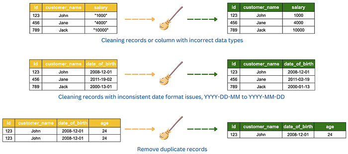
Data cleansing

Most of the data (raw) from source systems are dirty, incomplete and inconsistent. They may have unexpected format (such as JSON object), incorrect data types, missing values, duplicate records, repeated columns, inappropriate column names, etc. Data cleansing is the set of activities that you take to detect the inaccurate parts of the data and correcting all the issues found to arrive at a much cleaner datasets.

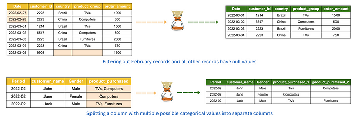
Data splitting

The objective of data splitting is to separate data into groups and structured format that is relevant to analyst or business user’s requirements. This may involve filtering out irrelevant columns and rows and also splitting information in a column that contains multiple categorical values.

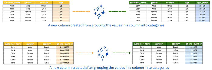
Data manipulation

Data manipulation is the process of modifying the existing data to make it more organized and readable for analysts and business users. Some examples of data manipulation are sorting the data in alphabetically for easy comprehension, masking confidential information such as bank account number and grouping data into bins, interval or categories for easier analysis.

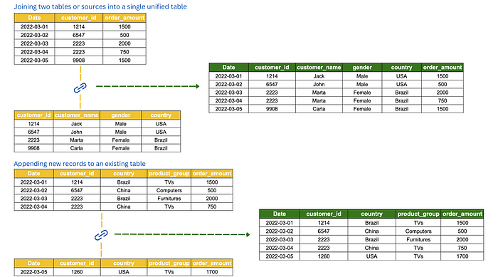
Data integration

A common task in data transformation is to combine data from multiple sources, to create a unified view of the data. Data integration may involve joining different data or tables into a single unified table and appending records or rows into a table.

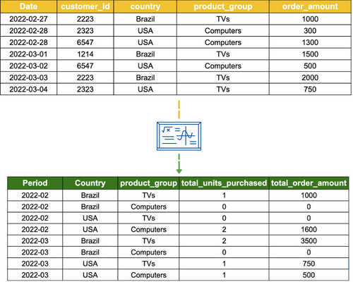
Data aggregation

Data aggregation is used when there is a need for data to be summarized for statistical analysis and reporting. This technique summarizes the measures (metrics) of your data against the dimensions (categorical information) in your data using aggregation functions such as SUM, COUNT and AVERAGE (in SQL). This allows business users to compare a wide range of data points, such as how sales differs across gender and country.

Data derivation

This technique creates a new data value from one or more contribution data values. As an example, a customer’s average spending is derived from his/her total spend divided by total transactions.

Data normalization

This technique is used on continuous data to scale the values into a smaller range so that they can be compared with each other. There are 2 popular methods to normalize your continuous data; Z-score normalization and Min-Max normalization.

File format optimizations

CSV, XML, JSON, and other types of plaintext files are commonly used to store structured and semi-structured data. These file formats are useful when manually exploring data, but there are much better, binary-based file formats to use for computer-based analytics. A common binary format that is optimized for read-heavy analytics is the Apache Parquet format. A common transformation is to convert plaintext files into an optimized format, such as Apache Parquet.

Within modern data lake environments, there are a number of file formats that can be used that are optimized for data analytics. From an analytics perspective, the most popular file format currently is Apache Parquet.

Parquet files are columnar-based, meaning that the contents of the file are physically stored to have data grouped by columns, rather than grouped by rows as with most file formats. (CSV files, for example, are physically stored to be grouped by rows.) As a result, queries that select a set of specific columns (rather than the entire row) do not need to read through all the data in the Parquet file to return a result, leading to performance improvements.

Parquet files also contain metadata about the data they store. This includes schema information (the data type for each column), as well as statistics such as the minimum and maximum value for a column contained in the file, the number of rows in the file, and so on.

A further benefit of Parquet files is that they are optimized for compression. A 1 TB dataset in CSV format could potentially be stored as 130 GB in Parquet format once compressed. Parquet supports multiple compression algorithms, although Snappy is the most widely used compression algorithm.

These optimizations result in significant savings, both in terms of storage space used and for running queries.

For example, the cost of an Amazon Athena query is based on the amount of compressed data scanned (at the time of writing, this cost was $5 per TB of scanned data). If only certain columns are queried of a Parquet file, then between the compression and only needing to read the data chunks for the specific columns, significantly less data needs to be scanned to resolve the query.

In a scenario where your data table is stored across perhaps hundreds of Parquet files in a data lake, the analytics engine is able to get further performance advantages by reading the metadata of the files. For example, if your query is just to count all the rows in a table, this information is stored in the Parquet file metadata, so the query doesn't need to actually scan any of the data. For this type of query, you will see that Athena indicates that 0 KB of data was scanned, therefore there is no cost for the query.

Or, if your query is for where the sales amount is above a specific value, the analytics engine can read the metadata for a column to determine the minimum and maximum values stored in the specific data chunk. If the value you are searching for is higher than the maximum value recorded in the metadata, then the analytics engine knows that it does not need to scan that specific column data chunk. This results in both cost savings and increased performance for queries.

Because of these performance improvements and cost savings, a very common transformation is to convert incoming files from their original format (such as CSV, JSON, XML, and so on) into the analytics-optimized Parquet format.

Data standardization

When building out a pipeline, we often load data from multiple different data sources, and each of those data sources may have different naming conventions for referring to the same item. For example, a field containing someone's birth date may be called DOB, dateOfBirth, birth_date, and so on. The format of the birth date may also be stored as mm/dd/yy, dd/mm/yyyy, or in a multitude of other formats.

One of the tasks we may want to do when optimizing data for analytics is to standardize column names, types, and formats. By having a corporate-wide analytic program, standard definitions can be created and adopted across all analytic projects in the organization.

Data quality checks

Another aspect of data transformation may be the process of verifying data quality and highlighting any ingested data that does not meet the expected quality standards.

Data partitioning

Partitioning and bucketing are used to maximize benefits while minimizing adverse effects. It can reduce the overhead of shuffling, the need for serialization, and network traffic. In the end, it improves performance, cluster utilization, and cost-efficiency.

Partition helps in localizing data and reducing data shuffling across the network nodes, reducing network latency, which is a major component of the transformation operation, thereby reducing the time of completion. A good partitioning strategy knows about data and its structure, and cluster configuration. Bad partitioning can lead to bad performance, mostly in 3 fields:

• Too many partitions regarding your cluster size and you won’t use efficiently your cluster. For example, it will produce intense task scheduling.
• Not enough partitions regarding your cluster size, and you will have to deal with memory and CPU issues: memory because your executor nodes will have to put high volume of data in memory (possibly causing OOM Exception), and CPU because compute across the cluster will be unequal.
• Skewed data in your partitions can occur. When a Spark task is executed in these partitioned, they will be distributed across executor slots and CPUs. If your partitions are unbalanced in terms of data volume, some tasks will run longer compared to others and will slow down the global execution time of the tasks (and a node will probably burn more CPU that others).

How to decide the partition key(s)?

• Choose low cardinality columns as partition columns (since a HDFS directory will be created for each partition value combination). Generally speaking, the total number of partition combinations should be less than 50K. (For example, don’t use partition keys such as roll_no, employee_ID etc. Instead use the state code, country code, geo_code, etc.)
• Choose the columns used frequently in filtering conditions.
• Use at most 2 partition columns as each partition column creates a new layer of directory.

Different methods that exist in PySpark

1. Repartitioning

The first way to manage partitions is the repartition operation. Repartitioning is the operation to reduce or increase the number of partitions in which the data in the cluster will be split. This process involves a full shuffle. Consequently, it is clear that repartitioning is an expensive process. In a typical scenario, most of the data should be serialized, moved, and deserialized.

repartitioned = df.repartition(8)

In addition to specifying the number of partitions directly, you can pass in the name of the column by which you want to partition the data.

repartitioned = df.repartition('country')

2. Coalesce

The second way to manage partitions is coalesce. This operation reduces the number of partitions and avoids a full shuffle. The executor can safely leave data on a minimum number of partitions, moving data only from redundant nodes. Therefore, it is better to use coalesce than repartition if you need to reduce the number of partitions.

coalesced = df.coalesce(2)

3. PartitionBy

partitionBy(cols) is used to define the folder structure of data. However, there is no specific control over how many partitions are going to be created. Different from the coalesce andrepartition functions, partitionBy effects the folder structure and does not have a direct effect on the number of partition files that are going to be created nor the partition sizes.

green_df \ 
    .write \ 
.partitionBy("pickup_year", "pickup_month") \ 
    .mode("overwrite") \ 
    .csv("data/partitions/partitionBy.csv", header=True)

Benefits of partitioning

Partitioning has several benefits apart from just query performance. Let's take a look at a few important ones.

1. Improving performance

Partitioning helps improve the parallelization of queries by splitting massive monolithic data into smaller, easily consumable chunks.

Apart from parallelization, partitioning also improves performance via data pruning. Using data pruning queries can ignore non-relevant partitions, thereby reducing the input/output (I/O) required for queries.

Partitions also help with the archiving or deletion of older data. For example, let's assume we need to delete all data older than 12 months. If we partition the data into units of monthly data, we can delete a full month's data with just a single DELETE command, instead of deleting all the files one by one or all the entries of a table row by row.

Let's next look at how partitioning helps with scalability.

2. Improving scalability

In the world of big data processing, there are two types of scaling: vertical and horizontal.

Vertical scaling refers to the technique of increasing the capacity of individual machines by adding more memory, CPU, storage, or network to improve performance. This usually helps in the short term, but eventually hits a limit beyond which we cannot scale.

The second type of scaling is called horizontal scaling. This refers to the technique of increasing processing and storage capacity by adding more and more machines to a cluster, with regular hardware specifications that are easily available in the market (commodity hardware). As and when the data grows, we just need to add more machines and redirect the new data to the new machines. This method theoretically has no upper bounds and can grow forever. Data lakes are based on the concept of horizontal scaling.

Data partitioning helps naturally with horizontal scaling. For example, let's assume that we store data at a per-day interval in partitions, so we will have about 30 partitions per month. Now, if we need to generate a monthly report, we can configure the cluster to have 30 nodes so that each node can process one day's worth of data. If the requirement increases to process quarterly reports (that is, reports every 3 months), we can just add more nodes---say, 60 more nodes to our original cluster size of 30 to process 90 days of data in parallel. Hence, if we can design our data partition strategy in such a way that we can split the data easily across new machines, this will help us scale faster.

Let's next look at how partitioning helps with data management.

3. Improving manageability

In many analytical systems, we will have to deal with data from a wide variety of sources, and each of these sources might have different data governance policies assigned to them. For example, some data might be confidential, so we need to restrict access to that; some might be transient data that can be regenerated at will; some might be logging data that can be deleted after a few months; some might be transaction data that needs to be archived for years; and so on. Similarly, there might be data that needs faster access, so we might choose to persist it on premium solid-state drive (SSD) stores and other data on a hard disk drive (HDD) to save on cost.

If we store such different sets of data in their own storage partitions, then applying separate rules---such as access restrictions, or configuring different data life cycle management activities such as deleting or archiving data, and so on---for the individual partitions becomes easy. Hence, partitioning reduces the management overhead, especially when dealing with multiple different types of data such as in a data lake.

Let's next look at how data partitioning helps with security.

4. Improving security

As we saw in the previous section about improving manageability, confidential datasets can have different access and privacy levels. Customer data will usually have the highest security and privacy levels. On the other hand, product catalogs might not need very high levels of security and privacy.

So, by partitioning the data based on security requirements, we can isolate the secure data and apply independent access-control and audit rules to those partitions, thereby allowing only privileged users to access such data.

Let's next look at how we can improve data availability using partitioning.

5. Improving availability

If our data is split into multiple partitions that are stored in different machines, applications can continue to serve at least partial data even if a few partitions are down. Only a subset of customers whose partitions went down might get impacted, while the rest of the customers will not see any impact. This is better than the entire application going down. Hence, physically partitioning the data helps improve the availability of services.

In general, if we plan our partition strategy correctly, the returns could be significant. I hope you have now understood the benefits of partitioning data. Let's next look at some partition strategies from a storage/files perspective.

Key Points

1. Do not partition by columns with high cardinality.
2. Partition by specific columns that are mostly used during filter and groupBy operations.
3. Even though there is no best number, it is recommended to keep each partition file size between 256MB to 1GB.
4. If you are increasing the number of partitions, use repartition()(performing full shuffle).
5. If you are decreasing the number of partitions, use coalesce() (minimizes shuffles).
6. Default no of partitions is equal to the number of CPU cores in the machine.
7. GroupByKey, ReduceByKey — by default this operation uses Hash Partitioning with default parameters.

A common optimization strategy for analytics is to partition the data, grouping the data at the physical storage layer by a field that is often used in queries. For example, if data is often queried by a date range, then data can be partitioned by a date field. If storing sales data, for example, all the sales transactions for a specific month would be stored in the same Amazon S3 prefix (which is much like a directory). When a query is run that selects all the data for a specific day, the analytic engine only needs to read the data in the directory that's storing data for the relevant month.

Another common approach for optimizing datasets for analytics is to partition the data, which relates to how the data files are organized in the storage system for a data lake.

Hive partitioning splits the data from a table to be grouped together in different folders, based on one or more of the columns in the dataset. While you can partition the data in any column, a common partitioning strategy that works for many datasets is to partition based on date.

For example, suppose you had sales data for the past four years from around the country, and you had columns in the dataset for Day, Month and Year. In this scenario, you could select to partition the data based on the Year column. When the data was written to storage, all the data for each of the past few years would be grouped together with the following structure:

datalake_bucket/year=2021/file1.parquet
datalake_bucket/year=2020/file1.parquet
datalake_bucket/year=2019/file1.parquet
datalake_bucket/year=2018/file1.parquet

If you then run a SQL query and include a WHERE Year = 2018 clause, for example, the analytics engine only needs to open up the single file in the datalake_bucket/year=2018 folder. Because less data needs to be scanned by the query, it costs less and completes quicker.

Deciding on which column to partition by requires that you have a good understanding of how the dataset will be used. If you partition your dataset by year but a majority of your queries are by the business unit (BU) column across all years, then the partitioning strategy would not be effective.

Queries you run that do not use the partitioned columns may also end up causing those queries to run slower if you have a large number of partitions. The reason for this is that the analytics engine needs to read data in all partitions, and there is some overhead in working between all the different folders. If there is no clear common query pattern, it may be better to not even partition your data. But if a majority of your queries use a common pattern, then partitioning can provide significant performance and cost benefits.

You can also partition across multiple columns. For example, if you regularly process data at the day level, then you could implement the following partition strategy:

datalake_bucket/year=2021/month=6/day=1/file1.parquet

This significantly reduces the amount of data to be scanned when queries are run at the daily level and also works for queries at the month or year level. However, another warning regarding partitioning is that you want to ensure that you don't end up with a large number of small files. The optimal size of Parquet files in a data lake is 128 MB–1 GB. The Parquet file format can be split, which means that multiple nodes in a cluster can process data from a file in parallel. However, having lots of small files requires a lot of overhead for opening, reading metadata, scanning data, and closing each file, and can significantly impact performance.

Partitioning is an important data optimization strategy and is based on how the data is expected to be used, either for the next transformation stage or for the final analytics stage. Determining the best partitioning strategy requires that you understand how the data will be used next.

Data denormalization

In traditional relational database systems, the data is normalized, meaning that each table contains information on a specific focused topic, and associated, or related, information is contained in a separate table. The tables can then be linked through the use of foreign keys.

For data lakes, combining the data from multiple tables into a single table can often improve query performance. Data denormalization takes two (or more) tables and creates a new table with data from both tables.

Data cataloging

Another important component that we should include in the transformation section of our pipeline architecture is the process of cataloging the dataset. During this process, we ensure all the datasets in the data lake are referenced in the data catalog and can add additional business metadata.

More Resources

1. https://www.fivetran.com/blog/what-is-data-transformation